4. Tutorial
4.1. Bulk Silicon
First, perform SCF calculation using Quantum Espresso (QE) with the following input file (e.g., scf.in):
&control
  prefix = 'prefix'
  calculation = 'scf'
  pseudo_dir = '/home/user/QE/pseudo_potential/'
  outdir = './'
  verbosity = 'high'
  disk_io = 'low'
/
&system
  ibrav = 2
  celldm(1) = 10.26
  nat = 2
  ntyp = 1
  nbnd = 10
  ecutwfc = 20.0
  occupations = 'fixed'
/
&electrons
  conv_thr = 1.0d-8
/
ATOMIC_SPECIES
  Si 1.0 Si.upf
ATOMIC_POSITIONS {alat}
  Si 0.00 0.00 0.00
  Si 0.25 0.25 0.25
K_POINTS {automatic}
   8 8 8 0 0 0
For running QE, please type
$ pw.x < scf.in > scf.out
For more information about QE, please see the QE website and keyword list.
In this calculation, the Ne-core pseudopotentials of silicon [1] taken from Pseudopotential Library is placed in pseudo_dir specified above and named as Si.upf.
Any calculation method in QE, such as DFT and HF, is acceptable as long as one can get one-elecron orbitals.
To obtain a band structure, we also need to perform band calculation using QE.
Warning
For QE band-structure calculation, please copy the directory where QE SCF calculation was performed, and perform QE band calculation there.
Namely, SCF and band calculations of QE should be performed in different directories (e.g., qescf directory and qeband directory).
This is to prevent output files from being overwritten. Thus, if you explicitly specify different outdir, you can use the same directory instead.
QE band calculation is performed with the following input file (e.g., band.in):
&control
  prefix = 'prefix'
  calculation = 'bands'
  pseudo_dir = '/home/user/QE/pseudo_potential/'
  outdir = './'
  verbosity = 'high'
  disk_io = 'low'
/
&system
  ibrav = 2
  celldm(1) = 10.26
  nat = 2
  ntyp = 1
  nbnd = 10
  ecutwfc = 20.0
  occupations = 'fixed'
/
&electrons
  conv_thr = 1.0d-8
/
ATOMIC_SPECIES
  Si 1.0 Si.upf
ATOMIC_POSITIONS {alat}
  Si 0.00 0.00 0.00
  Si 0.25 0.25 0.25
K_POINTS {crystal_b}
3
 0.5 0.5 0.0 20
 0.0 0.0 0.0 20
 0.5 0.0 0.0 0
and type
$ pw.x < band.in > band.out
Next, perform SCF calculation using TC++ with the following input file, input.in,
calc_method   HF  # change here for different methods (TC, BITC)
calc_mode     SCF
pseudo_dir    /home/user/QE/pseudo_potential
qe_save_dir   /home/user/where_QE_SCFcalc_was_performed/prefix.save
smearing_mode fixed
where pseudo_dir and qe_save_dir shoud be appropriately specified. Without MPI parallelization, simply typing
$ ./tc++
will work if tc++ is placed in this folder. However, we recommend to use MPI parallelization since this calculation requires \(O(1)\) core hours for HF and \(O(10)\) (- \(O(100)\)) core hours for (BI)TC.
See How to use for more details about how to run TC++.
After SCF calculation, we should check whether ‘convergence is achieved!’ is shown in output.out.
If the convergence is not achieved, we can restart calculation using input.in with the following line added:
restarts true
However, it is often difficult to achieve convergence in BITC calculations.
While convergence can be improved by increasing the number of k-points and/or max_num_blocks_david in input.in,
we did not do so in this tutorial.
To improve the convergence, it is also effective to reduce mixing_beta with mixes_density_matrix = true.
Band structures shown later were obtained without taking these ways or restarting calculation.
Finally, we perform the band calculation.
Warning
For TC++ band-structure calculation, please copy the directory where TC++ SCF calculation was performed, and perform TC++ band calculation there.
SCF and band calculations of TC++ should also be performed in different directories because the input and output file names, input.in and output.out, are in common between two calculations.
Required input.in for band calculation is as follows,
calc_method   HF  # change here for different methods (TC, BITC)
calc_mode     BAND
pseudo_dir    /home/user/QE/pseudo_potential
qe_save_dir   /home/user/where_QE_BANDcalc_was_performed/prefix.save
smearing_mode fixed
Note that qe_save_dir is different from that used in SCF calculation.
The band calculation requires tc_energy_scf.dat, tc_wfc_scf.dat, and tc_scfinfo.dat, which were dumped in TC++ SCF calculation (see How to use for details). These files should be placed in the directory where TC++ band calculation runs. A command for running TC++ is the same as SCF: ./tc++ for non-MPI-parallelized calculation, but we strongly recommend to use MPI parallelization.
Users can apply restarts = true also for BAND calculation if necessary (e.g., when band calculation stops before convergence is achieved).
A small error will remain in these tutorial calculations of the TC and BITC methods, which can be reduced by increasing the number of k-points and/or
changing the choice of the band k-points (See Tips & FAQ). The calculated band eigenvalues are dumped in tc_bandplot.dat, as shown below (Note: PBE-GGA band structure was drawn using QE).
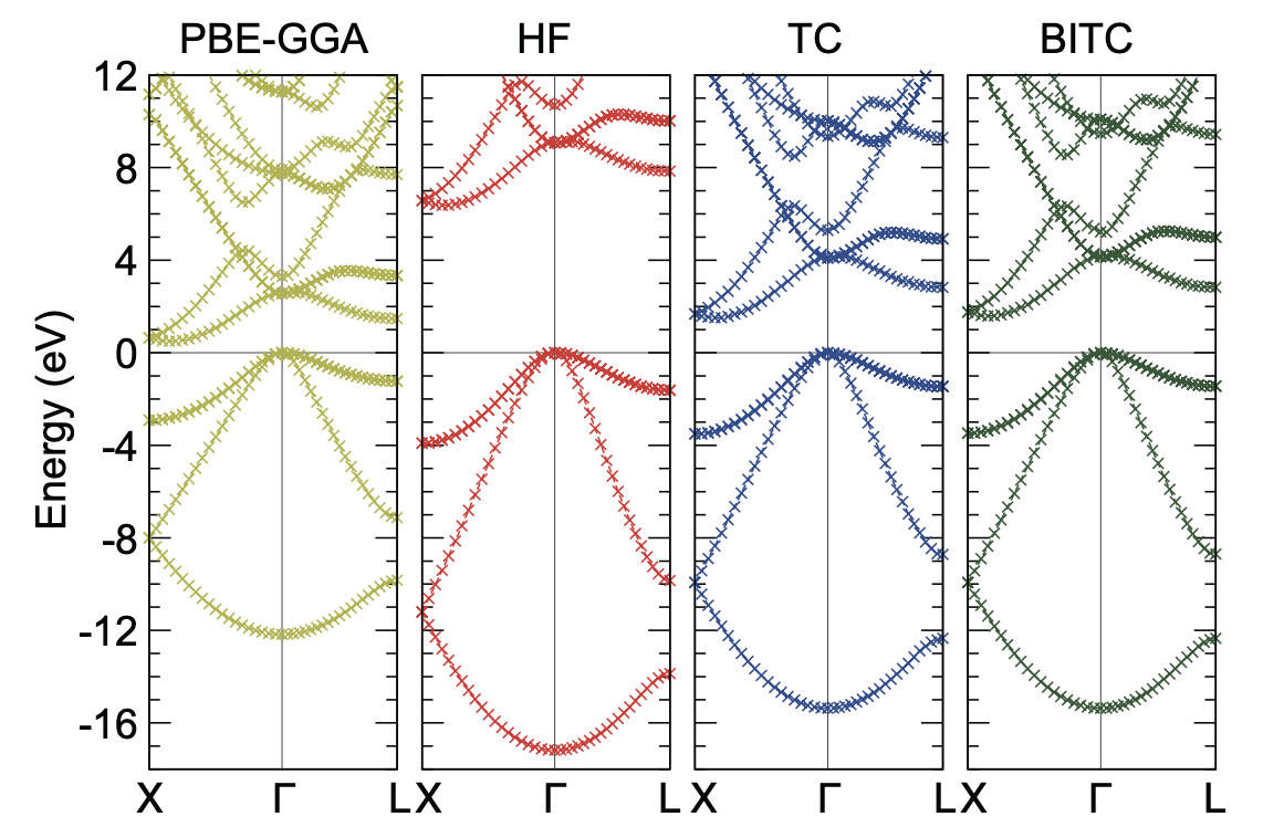
For plotting these band structures, we used gnuplot and typed EF = 4..... (please fill in the value of the Fermi energy (EF) shown in tc_bandplot.dat) and p 'tc_bandplot.dat' u 4:($5-EF) w linesp.
Here, EF was subtracted from the band eigenvalues. When smearing_mode = fixed is used, EF is the valence-band maximum energy.
When smearing_mode = gaussian is used, EF is the chemical potential (Fermi level) used for the Gaussian smearing.
Users can also perform fake-SCF calculation, where SCF and BAND calculations are simultaneously performed by specifying the k-points with an appropriate weight. For this purpose, please perform QE calculation using the following input file (for a \(4\times 4\times 4\) k-mesh)
&control
  prefix = 'prefix'
  calculation = 'scf'
  pseudo_dir = '/home/user/QE/pseudo_potential/'
  outdir = './'
  verbosity = 'high'
  disk_io = 'low'
/
&system
  ibrav = 2
  celldm(1) = 10.26
  nat = 2
  ntyp = 1
  nbnd = 10
  ecutwfc = 20.0
  occupations = 'fixed'
/
&electrons
  conv_thr = 1.0d-8
/
ATOMIC_SPECIES
  Si 1.0 Si.upf
ATOMIC_POSITIONS {alat}
  Si 0.00 0.00 0.00
  Si 0.25 0.25 0.25
K_POINTS {crystal}
19
  0.0 0.0 0.0 0.03125
  0.0 0.0 0.25 0.25
  0.0 0.0 -0.5 0.125
  0.0 0.25 0.25 0.1875
  0.0 0.25 -0.5 0.75
  0.0 0.25 -0.25 0.375
  0.0 -0.5 -0.5 0.09375
  0.25 -0.5 -0.25 0.1875
  0.0 0.0 0.0 0.0
  0.05 0.0 0.0 0.0
  0.1 0.0 0.0 0.0
  0.15 0.0 0.0 0.0
  0.2 0.0 0.0 0.0
  0.25 0.0 0.0 0.0
  0.3 0.0 0.0 0.0
  0.35 0.0 0.0 0.0
  0.4 0.0 0.0 0.0
  0.45 0.0 0.0 0.0
  0.5 0.0 0.0 0.0
and then perform SCF calculation with TC++, which gives the SCF and BAND eigenvalues simultaneously.
However, we do not recommend this way by the following reasons: band eigenvalues are not checked for convergence in this calculation (see energy_tolerance
in Input parameters in input.in), and computational cost becomes expensive because the computation time is proportional to the square of the number of k-points.
Note that tc_bandplot.dat is not dumped in the fake-SCF procedure since calc_mode = SCF.
4.2. Homogeneous Electron Gas
TC++ also supports calculation of homogeneous electron gas. First, perform SCF calculation using QE with the following input file,
&control
  prefix = 'prefix'
  calculation = 'scf'
  pseudo_dir = '/home/user/QE/pseudo_potential/'
  outdir = './'
  verbosity = 'high'
  disk_io = 'low'
/
&system
  ibrav = 1
  celldm(1) = 7.67663317071 ! Bohr
  nat = 1
  ntyp = 1
  nbnd = 20
  ecutwfc = 20.0
  occupations = 'smearing'
  smearing = 'gauss'
  degauss = 0.03 ! Ry
/
&electrons
  conv_thr = 1.0d-8
/
ATOMIC_SPECIES
  Si 1.0 Si.upf
ATOMIC_POSITIONS {alat}
  Si 0.00 0.00 0.00
K_POINTS {automatic}
 12 12 12 0 0 0
where the pseudopotential file, Si.upf, placed in pseudo_dir is used because calculation of homogeneous electron gas is not implemented in QE. Four valence electrons in the simple-cubic lattice with this lattice constant corresponds to the \(r_s\) parameter of 3 Bohr in electron gas. For a band-structure plot, perform the band calculation using QE with the following input file,
&control
  prefix = 'prefix'
  calculation = 'bands'
  pseudo_dir = '/home/user/QE/pseudo_potential/'
  outdir = './'
  verbosity = 'high'
  disk_io = 'low'
/
&system
  ibrav = 1
  celldm(1) = 7.67663317071 ! Bohr
  nat = 1
  ntyp = 1
  nbnd = 20
  ecutwfc = 20.0
  occupations = 'smearing'
  smearing = 'gauss'
  degauss = 0.03 ! Ry
/
&electrons
  conv_thr = 1.0d-8
/
ATOMIC_SPECIES
  Si 1.0 Si.upf
ATOMIC_POSITIONS {alat}
  Si 0.00 0.00 0.00
K_POINTS {tpiba_b}
3
-0.5 -0.5 -0.5 20
0.0 0.0 0.0 20
0.5 0.0 0.0 0
Then, perform SCF calculation using TC++ with the following input.in,
calc_method     FREE  # change here for different methods (HF, TC)
calc_mode       SCF   # SCF or BAND
pseudo_dir      /home/user/QE/pseudo_potential
qe_save_dir     /home/user/where_QE_SCFcalc_was_performed/prefix.save
smearing_mode   gaussian
smearing_width  0.02  # in Ht.
is_heg          true
and perform band calculation by changing calc_mode and qe_save_dir in the above input.in.
Note that qe_save_dir in band calculation should be the directory where QE band calculation (not SCF!) was performed. The calculated band structures are shown below.
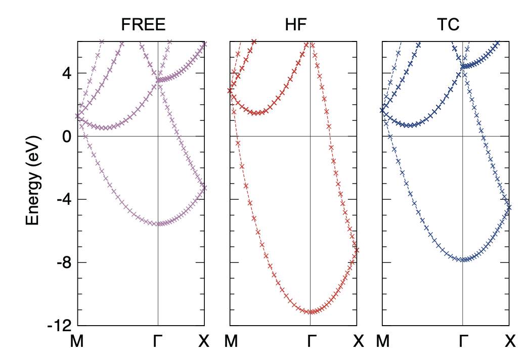
One notable feature here is that the HF band structure has a well-known singularity at the Fermi energy: the density of states becomes zero at the Fermi energy with a logarithmic singularity. This is due to a lack of the screening effect of the electron-electron interaction in the Hartree-Fock theory. As a result, the HF band structure is quite dispersive near the Fermi energy. On the other hand, the TC band structure does not have this kind of unphysical behavior thanks to the Jastrow factor that includes the screening effect. Note that BITC should offer the same result as TC because left and right one-electron orbitals are the same plane waves for homogeneous electron gas.
Users can use a different value for the lattice type, the atomic species, and the lattice constant. The subsequent TC++ run only uses the number of electrons and the periodic cell. Since TC++ can use crystal symmetries existing in the QE input, high-symmetry structure is preferable for efficient computation.